2. The BQL Language
This part describes the use of the BQL Language in SensorBee. It starts with describing the general syntax of BQL, then explain how to create the structures for data in-/output and stateful operations. After that, the general processing model and the remaining BQL query types are explained. Finally, a list of operators and functions that can be used in BQL expressions is provided.
2.1. BQL Syntax
2.1.1. Lexical Structure
BQL has been designed to be easy to learn for people who have used SQL before. While keywords and commands differ in many cases, the basic structure, set of tokens, operators etc. is the same. For example, the following is (syntactically) valid BQL input:
SELECT RSTREAM given_name, last_name FROM persons [RANGE 1 TUPLES] WHERE age > 20;

CREATE SOURCE s TYPE fluentd WITH host="example.com", port=12345;

INSERT INTO file FROM data;
This is a sequence of three commands, one per line (although this is not required; more than one command can be on a line, and commands can span multiple lines where required). Additionally, comments can occur in BQL input. They are effectively equivalent to whitespace.
The type of commands that can be used in BQL is described in Input/Output/State Definition and Queries.
2.1.1.1. Identifiers and Keywords
Tokens such as SELECT, CREATE, or INTO in the example above are examples of keywords, that is, words that have a fixed meaning in the BQL language.
The tokens persons and file are examples of identifiers.
They identify names of streams, sources, or other objects, depending on the command they are used in.
Therefore they are sometimes simply called “names”.
Keywords and identifiers have the same lexical structure, meaning that one cannot know whether a token is an identifier or a keyword without knowing the language.
BQL identifiers and keywords must begin with a letter (a-z).
Subsequent characters can be letters, underscores, or digits (0-9).
Keywords and unquoted identifiers are in general case insensitive.
However, there is one important difference between SQL and BQL when it comes to “column identifiers”.
In BQL, there are no “columns” with names that the user can pick herself, but “field selectors” that describe the path to a value in a JSON-like document imported from outside the system.
Therefore field selectors are case-sensitive (in order to be able to deal with input of the form {"a": 1, "A": 2}) and also there is a form that allows to use special characters; see Field Selectors for details.
Note
There is a list of reserved words that cannot be used as identifiers to avoid confusion. This list can be found at https://github.com/sensorbee/sensorbee/blob/master/core/reservedwords.go. However, this restriction does not apply to field selectors.
2.1.1.2. Constants
There are multiple kinds of implicitly-typed constants in BQL: strings, decimal numbers (with and without fractional part) and booleans. Constants can also be specified with explicit types, which can enable more accurate representation and more efficient handling by the system. These alternatives are discussed in the following subsections.
String Constants
A string constant in BQL is an arbitrary sequence of characters bounded by double quotes ("), for example "This is a string".
To include a double-quote character within a string constant, write two adjacent double quotes, e.g., "Dianne""s horse".
No escaping for special characters is supported at the moment, but any valid UTF-8 encoded byte sequence can be used. See the string data type reference for details.
Numeric Constants
There are two different numeric data types in BQL, int and float, representing decimal numbers without and with fractional part, respectively.
An int constant is written as
[-]digits
A float constant is written as
[-]digits.digits
Scientific notation (1e+10) as well as Infinity and NaN cannot be used in BQL statements.
Some example of valid numerical constants:
42
3.5
-36
See the type references for int and float for details.
Note
For some operations/functions it makes a difference whether int or float is used (e.g., 2/3 is 0, but 2.0/3 is 0.666666).
Be aware of that when writing constants in BQL statements.
Boolean Constants
There are two keywords for the two possible boolean values, namely true and false.
See the bool data type reference for details.
2.1.1.3. Operators
An operator is a sequence of the items from the following list:
+
-
*
/
<
>
=
!
%
See the chapter on Operators for the complete list of operators in BQL. There are no user-defined operators at the moment.
2.1.1.4. Special Characters
Some characters that are not alphanumeric have a special meaning that is different from being an operator. Details on the usage can be found at the location where the respective syntax element is described. This section only exists to advise the existence and summarize the purposes of these characters.
- Parentheses (
()) have their usual meaning to group expressions and enforce precedence. In some cases parentheses are required as part of the fixed syntax of a particular BQL command. - Brackets (
[]) are used in Array Constructors and in Field Selectors, as well as in Stream-to-Relation Operators. - Curly brackets (
{}) are used in Map Constructors - Commas (
,) are used in some syntactical constructs to separate the elements of a list. - The semicolon (
;) terminates a BQL command. It cannot appear anywhere within a command, except within a string constant or quoted identifier. - The colon (
:) is used to separate stream names and field selectors, and within field selectors to select array slices (see Extended Descend Operators). - The asterisk (
*) is used in some contexts to denote all the fields of a table row (see Notes on Wildcards). It also has a special meaning when used as the argument of an aggregate function, namely that the aggregate does not require any explicit parameter. - The period (
.) is used in numeric constants and to denote descend in field selectors.
2.1.1.5. Comments
A comment is a sequence of characters beginning with double dashes and extending to the end of the line, e.g.:
-- This is a standard BQL comment
C-style (multi-line) comments cannot be used.
2.1.1.6. Operator Precedence
The following table shows the operator precedence in BQL:
| Operator/Element | Description |
|---|---|
:: |
typecast |
- |
unary minus |
* / % |
multiplication, division, modulo |
+ - |
addition, subtraction |
IS |
IS NULL etc. |
| (any other operator) | e.g., || |
= != <> <= < >= > |
comparison operator |
NOT |
logical negation |
AND |
logical conjunction |
OR |
logical disjunction |
2.1.2. Value Expressions
Value expressions are used in a variety of contexts, such as in the target list or filter condition of the SELECT command.
The expression syntax allows the calculation of values from primitive parts using arithmetic, logical, set, and other operations.
A value expression is one of the following:
- A constant or literal value
- A field selector
- A row metadata reference
- An operator invocation
- A function call
- An aggregate expression
- A type cast
- An array constructor
- A map constructor
- Another value expression in parentheses (used to group subexpressions and override precedence)
The first option was already discussed in Constants. The following sections discuss the remaining options.
2.1.2.1. Field Selectors
In SQL, each table has a well-defined schema with columns, column names and column types. Therefore, a column name is enough to check whether that column exists, what type it has and if the type that will be extracted matches the type expected by the surrounding expression.
In BQL, each row corresponds to a JSON-like object, i.e., a map with string keys and values that have one of several data types (see Data Types and Conversions). In particular, nested maps and arrays are commonplace in the data streams used with BQL. For example, a row could look like:
{"ids": [3, 17, 21, 5],
 "dists": [
  {"other": "foo", "value": 7},
  {"other": "bar", "value": 3.5}
 ],
 "found": true}
To deal with such nested data structures, BQL uses a subset of JSON Path to address values in a row.
Basic Descend Operators
In general, a JSON Path describes a path to a certain element of a JSON document. Such a document is looked at as a rooted tree and each element of the JSON Path describes how to descend from the current node to a node one level deeper, with the start node being the root. The basic rules are:
If the current node is a map, then
.child_key
or
["child_key"]
mean “descend to the child node with the key
child_key”. The second form must be used if the key name has a non-identifier shape (e.g., contains spaces, dots, brackets or similar). It is an error if the current node is not a map. It is an error if the current node does not have such a child node.If the current node is an array, then
[k]
means “descend to the (zero-based) \(k\)-th element in the array”. Negative indices count from the end end of the array (as in Python). It is an error if the current node is not an array. It is an error if the given index is out of bounds.
The first element of a JSON Path must always be a “map access” component (since the document is always a map) and the leading dot must be omitted.
For example, ids[1] in the document given above would return 17, dists[-2].other would return foo and just dists would return the array [{"other": "foo", "value": 7}, {"other": "bar", "value": 3.5}].
Extended Descend Operators
There is limited support for array slicing and recursive descend:
If the current node is a map or an array, then
..child_key
returns an array of all values below the current node that have the key
child_key. However, once a node with keychild_keyhas been found, it will be returned as is, even if it may possibly itself contain that key again.This selector cannot be used as the first component of a JSON Path. It is an error if the current node is not a map or an array. It is not an error if there is no child element with the given key.
If the current node is an array, then
[start:end]
returns an array of all values with the indexes in the range \([\text{start}, \text{end}-1]\). One or both of
startandendcan be omitted, meaning “from the first element” and “until the last element”, respectively.[start:end:step]
returns an array of all elements with the indexes \([\text{start}, \text{start}+\text{step}, \text{start}+2\cdot\text{step}, \cdot\cdot\cdot, \text{end}-1]\) if
stepis positive, or \([\text{start}, \text{start}-\text{step}, \text{start}-2\cdot\text{step}, \cdot\cdot\cdot, \text{end}+1]\) if it is negative. (This description is only true for positive indices, but in fact also negative indices can be used, again counting from the end of the array.) In general, the behavior has been implemented to be very close to Python’s list slicing.These selectors cannot be used as the first component of a JSON Path. It is an error if it can be decided independent of the input data that the specified values do not make sense (e.g.,
stepis 0, orendis larger thanstartbutstepis negative), but slices that will always be empty (e.g.,[2:2]) are valid. Also, if it depends on the input data whether a slice specification is valid or not (e.g.,[4:-4]) it is not an error, but an empty array is returned.If the slicing or recursive descend operators are followed by ordinary JSON Path operators as described before, their meaning changes to ”... for every element in the array”. For example,
list[1:3].foohas the same result as[list[1].foo, list[2].foo, list[3].foo](except that the latter would fail iflistis not long enough) or a Python list comprehension such as[x.foo for x in list[1:3]]. However, it is not possible to chain multiple list-returning operators:list[1:3]..fooorfoo..bar..hogeare invalid.
Examples
Given the input data
{
    "foo": [
        {"hoge": [
            {"a": 1, "b": 2},
            {"a": 3, "b": 4} ],
         "bar": 5},
        {"hoge": [
            {"a": 5, "b": 6},
            {"a": 7, "b": 8} ],
         "bar": 2},
        {"hoge": [
            {"a": 9, "b": 10} ],
         "bar": 8}
    ],
    "nantoka": {"x": "y"}
}
the following table is supposed to illustrate the effect of various JSON Path expressions.
| Path | Result |
|---|---|
nantoka |
{"x": "y"} |
nantoka.x |
"y" |
nantoka["x"] |
"y" |
foo[0].bar |
5 |
foo[0].hoge[-1].a |
3 |
["foo"][0]["hoge"][-1]["a"] |
3 |
foo[1:2].bar |
[2, 8] |
foo..bar |
[5, 2, 8] |
foo..hoge[0].b |
[2, 6, 10] |
2.1.2.2. Row Metadata References
Metadata is the data that is attached to a tuple but which cannot be accessed as part of the normal row data.
Tuple Timestamp
At the moment, the only metadata that can be accessed from within BQL is a tuple’s system timestamp (the time that was set by the source that created it).
This timestamp can be accessed using the ts() function.
If multiple streams are joined, a stream prefix is required to identify the input tuple that is referred to, i.e.,
stream_name:ts()
2.1.2.3. Operator Invocations
There are three possible syntaxes for an operator invocation:
expression  operator  expression

operator  expression

expression  operator
See the section Operators for details.
2.1.2.4. Function Calls
The syntax for a function call is the name of a function, followed by its argument list enclosed in parentheses:
function_name([expression [, expression ... ]])
For example, the following computes the square root of 2:
sqrt(2);
The list of built-in functions is described in section Functions.
2.1.2.5. Aggregate Expressions
An aggregate expression represents the application of an aggregate function across the rows selected by a query. An aggregate function reduces multiple inputs to a single output value, such as the sum or average of the inputs. The syntax of an aggregate expression is the following:
function_name(expression [, ... ] [ order_by_clause ])
where function_name is a previously defined aggregate and expression is any value expression that does not itself contain an aggregate expression.
The optional order_by_clause is described below.
In BQL, aggregate functions can take aggregate and non-aggregate parameters.
For example, the string_agg function can be called like
string_agg(name, ", ")
to return a comma-separated list of all names in the respective group. However, the second parameter is not an aggregation parameter, so for a statement like
SELECT RSTREAM string_agg(name, sep) FROM ...
sep must be mentioned in the GROUP BY clause.
For many aggregate functions (e.g., sum or avg), the order of items in the group does not matter.
However, for other functions (e.g., string_agg) the user has certain expectations with respect to the order that items should be fed into the aggregate function.
In this case, the order_by_clause with the syntax
ORDER BY expression [ASC | DESC] [ , expression [ASC | DESC] ... ]
can be used. The rows that are fed into the aggregate function are sorted by the values of the given expression in ascending (default) or descending mode. For example,
string_agg(first_name || " " || last_name, "," ORDER BY last_name)
will create a comma-separated list of names, ordered ascending by the last name.
See Aggregate Functions for a list of built-in aggregate functions.
2.1.2.6. Type Casts
A type cast specifies a conversion from one data type to another. BQL accepts two equivalent syntaxes for type casts:
CAST(expression AS type)
expression::type
When a cast is applied to a value expression, it represents a run-time type conversion. The cast will succeed only if a suitable type conversion operation has been defined, see Conversions.
2.1.2.7. Array Constructors
An array constructor is an expression that builds an array value using values for its member elements.
A simple array constructor consists of a left square bracket [, a list of expressions (separated by commas) for the array element values, and finally a right square bracket ].
For example:
SELECT RSTREAM [7, 2 * stream:a, true, "blue"] FROM ...
Each element of the array can have a different type. In particular, the wildcard is also allowed as an expression and will include the whole current row (i.e., a map) as an array element.
Note
Single-element arrays of strings could also be interpreted as JSON Paths and are therefore required to have a trailing comma after their only element: ["foo",]
2.1.2.8. Map Constructors
A map constructor is an expression that builds a map value using string keys and arbitrary values for its member elements.
A simple map constructor consists of a left curly bracket {, a list of "key": value pairs (separated by commas) for the map elements, and finally a right curly bracket }.
For example:
SELECT RSTREAM {"a_const": 7, "prod": 2 * stream:a} FROM ...
The keys must be string literals (i.e., they cannot be computed expressions); in particular they must be written using double quotes. The values can be arbitrary expressions, including a wildcard.
2.1.2.9. Expression Evaluation Rules
The order of evaluation of subexpressions is not defined. In particular, the inputs of an operator or function are not necessarily evaluated left-to-right or in any other fixed order.
Furthermore, if the result of an expression can be determined by evaluating only some parts of it, then other subexpressions might not be evaluated at all. For instance, if one wrote:
true OR somefunc()
then somefunc() would (probably) not be called at all.
The same would be the case if one wrote:
somefunc() OR true
Note that this is not the same as the left-to-right “short-circuiting” of Boolean operators that is found in some programming languages.
2.1.3. Calling Functions
BQL allows functions to be called using only the positional notation. In positional notation, a function call is written with its argument values in the same order as they are defined in the function declaration. Therefore, while some parameters of a function can be optional, these parameters can only be omitted at the end of the parameter list.
For example,
log(100)
log(100, 2)
are both valid function calls computing the logarithm of a function. The first one uses the default value 10 for the logarithm base, the second one uses the given value 2.
2.2. Input/Output/State Definition
To process streams of data, that data needs to be imported into SensorBee and the processing results have to be exported from it. This chapter introduces input and output components in BQL. It also describes how BQL supports stateful data processing using user-defined states (UDSs).
2.2.1. Data Input
BQL inputs a stream of data using a source. A source receives data defined and generated outside SensorBee, converts that data into tuples, and finally emits tuples for further processing. This section describes how a source can be created, operated, and dropped.
2.2.1.1. Creating a Source
A source can be created using the CREATE SOURCE statement.
CREATE SOURCE logs TYPE file WITH path = "access_log.jsonl";
In this example, a source named logs is created and it has the type
file. The file source type has a required parameter called path. The
parameter is specified in the WITH clause. Once a source is created, other
components described later can read tuples from the source and compute results
based on them.
When multiple parameters are required, they should be separated by commas:
CREATE SOURCE src TYPE some_type
    WITH param1 = val1, param2 = val2, param3 = val3;
Each source type has its own parameters and there is no parameter that is common to all source types.
Source types can be registered to the SensorBee server as plugins. To learn how to develop and register a source plugin, see Source Plugins.
Built-in Sources
BQL has a number of built-in source types.
file
Thefiletype provides a source that inputs tuples from an existing file.
node_statuses
Thenode_statusessource periodically emits tuples with information about nodes in a topology. The status includes connected nodes, number of tuples emitted from or written to the node, and so on.
edge_statuses
Theedge_statusessource periodically emits tuples with information about each edge (a.k.a. pipe) that connects a pair of nodes. Although this information is contained in tuples emitted fromnode_statusessource, theedge_statusessource provides more edge-centric view of IO statuses.
dropped_tuples
Thedropped_tuplesemits tuples dropped from a topology. It only reports once per tuple. Tuples are often dropped from a topology because a source or a stream is not connected to any other node or aSELECTstatement tries to look up a nonexistent field of a tuple.
2.2.1.2. Pausing and Resuming a Source
By default, a source starts emitting tuples as soon as it is created. By adding
the PAUSED keyword to the CREATE SOURCE statement, it creates a source
that is paused on startup:
CREATE PAUSED SOURCE logs TYPE file WITH path = "access_log.jsonl";
The RESUME SOURCE statement makes a paused source emit tuples again:
RESUME SOURCE logs;
The statement takes the name of the source to be resumed.
A source can be paused after it is created by the PAUSE SOURCE statement:
PAUSE SOURCE logs;
The statement also takes the name of the source to be paused.
Not all sources support PAUSE SOURCE and RESUME SOURCE statements.
Issuing statements to those sources results in an error.
2.2.1.3. Rewinding a Source
Some sources can be rewound, that is, they emit tuples again starting from the beginning. The REWIND SOURCE statement rewinds a source if the source supports the statement:
REWIND SOURCE logs;
The statement takes the name of the source to be rewound. Issuing the statement to sources that don’t support rewinding results in an error.
2.2.1.4. Dropping a Source
The DROP SOURCE statement drops (i.e. removes) a source from a topology:
DROP SOURCE logs;
The statement takes the name of the source to be dropped. Other nodes in a topology cannot refer to the source once it’s dropped. Also, nodes connected to a source may be stopped cascadingly when the source gets dropped.
2.2.2. Data Output
Results of tuple processing need to be emitted to systems or services running outside the SensorBee server in order to work with them as part of a larger system. A sink receives the results of computations performed within the SensorBee server and sends them to the outside world. This section explains how sinks are operated in BQL.
2.2.2.1. Creating a Sink
A sink can be created by the CREATE SINK statement:
CREATE SINK filtered_logs TYPE file WITH path = "filtered_access_log.jsonl";
The statement is very similar to the CREATE SOURCE statement. It takes the
name of the new sink, its type, and parameters. Multiple parameters can also be
provided as a list separated by commas. Each sink type has its own parameters
and there is no parameter that is common to all sink types.
Sink types can also be registered to the SensorBee server as plugins. To learn how to develop and register a sink plugin, see Sink Plugins.
Built-in Sinks
BQL has a number of built-in sink types.
file
Thefiletype provides a sink that writes tuples to a file.
stdout
Astdoutsink writes output tuples to stdout.
uds
Audssink passes tuples to user-defined states, which is described later.
2.2.2.2. Writing Data to a Sink
The INSERT INTO statement writes data to a sink:
INSERT INTO filtered_logs FROM filtering_stream;
The statement takes the name of sink to be written and the name of a source or a stream, which will be described in following chapters.
2.2.3. Stateful Data Processing
SensorBee supports user-defined states (UDSs) to perform stateful streaming data processing. Such processing includes not only aggregates such as counting but also machine learning, adaptive sampling, and so on. In natural language processing, dictionaries or configurations for tokenizers can also be considered as states.
This section describes operations involving UDSs. Use cases of UDSs are described in the tutorials and how to develop a custom UDS is explained in the server programming part.
2.2.3.1. Creating a UDS
A UDS can be created using the CREATE STATE statement:
CREATE STATE age_classifier TYPE jubaclassifier_arow
    WITH label_field = "age", regularization_weight = 0.001;
This statement creates a UDS named age_classifier with the type
jubaclassifier_arow. It has two parameters: label_field and
regularization_weight. Each UDS type has its own parameters and there is no
parameter that is common to all UDS types.
A UDS is usually used via user-defined functions (UDFs) that know about the internals of a specific UDS type. See server programming part for details.
2.2.3.2. Saving a State
The SAVE STATE statement persists a UDS:
SAVE STATE age_classifier;
The statement takes the name of the UDS to be saved. After the statement is issued, SensorBee saves the state based on the given configuration. The location and the format of saved data depend on the run-time configuration and are unknown to users.
The SAVE STATE statement may take a TAG to support versioning of the
saved data:
SAVE STATE age_classifier TAG initial;
-- or
SAVE STATE age_classifier TAG trained;
When the TAG clause is omitted, default will be the default tag name.
2.2.3.3. Loading a State
The LOAD STATE loads a UDS that was previously saved with the
SAVE STATE statement:
LOAD STATE age_classifier TYPE jubaclassifier_arow;
The statement takes the name of the UDS to be loaded and its type name.
The LOAD STATE statements may also take a TAG:
LOAD STATE age_classifier TYPE jubaclassifier_arow TAG initial;
-- or
LOAD STATE age_classifier TYPE jubaclassifier_arow TAG trained;
The UDS needs to have been saved with the specified tag before. When the TAG
clause is omitted, it’s same as:
LOAD STATE age_classifier TYPE jubaclassifier_arow TAG default;
The LOAD STATE statement fails if no saved state with the given name
and type exists. In that case, to avoid failure and instead create a new
“empty” instance, the OR CREATE IF NOT SAVED clause can be added:
LOAD STATE age_classifier TYPE jubaclassifier_arow
    OR CREATE IF NOT SAVED
        WITH label_field = "age", regularization_weight = 0.001;
If there is a saved state, this statement will load it, otherwise create a
new state with the given parameters. This variant, too, can be used with
the TAG clause:
LOAD STATE age_classifier TYPE jubaclassifier_arow TAG trained
    OR CREATE IF NOT SAVED
        WITH label_field = "age", regularization_weight = 0.001;
2.2.3.4. Dropping a State
The DROP STATE statement drops a UDS from a topology:
DROP STATE age_classifier;
The statement takes the name of the UDS to be dropped. Once a UDS is dropped, it can no longer be referred to by any statement unless it is cached somewhere.
2.3. Queries
The previous chapters described how to define data sources and sinks to communicate with the outside world. Now it is discussed how to transform the data stream from those sources and write it to the defined sinks - that is, how to actually process data.
2.3.1. Processing Model
2.3.1.1. Overview
The processing model in BQL is similar to what is explained in [cql]. In this model, each tuple in a stream has the shape \((t, d)\), where \(t\) is the original timestamp and \(d\) the data contained.
In order to execute SQL-like queries, a finite set of tuples from the possibly unbounded stream, a relation, is required.
In the processing step at time \(t^*\), a stream-to-relation operator \(R\) that converts a certain set of tuples in the stream to a relation \(R(t^*)\) is used.
This relation is then processed with a relation-to-relation operator \(O\) that is expressed in a form very closely related to an SQL SELECT statement.
Finally, a relation-to-stream operator \(S\) will emit certain rows from the output relation \(O(R(t^*))\) into the output stream, possibly taking into account the results of the previous execution step \(O(R(t^*_{\text{prev}}))\).
This process is illustrated in the following figure:
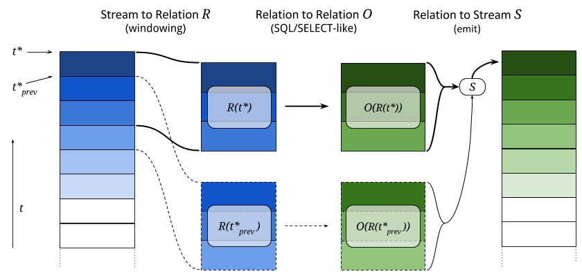
This three-step pipeline is executed for each tuple, but only for one tuple at a time. Therefore, during execution there is a well-defined “current tuple”. This also means that if there is no tuple in the input stream for a long time, transformation functions will not be called.
Now the kind of stream-to-relation and relation-to-stream operators that can be used in BQL is explained.
2.3.1.2. Stream-to-Relation Operators
In BQL, there are two different stream-to-relation operators, a time-based one and a tuple-based one.
They are also called “window operators”, since they define a sliding window on the input stream.
In terms of BQL syntax, the window operator is given after a stream name in the FROM clause within brackets and using the RANGE keyword, for example:
... FROM events [RANGE 5 SECONDS] ...
... FROM data [RANGE 10 TUPLES] ...
... FROM left [RANGE 2 SECONDS], right [RANGE 5 TUPLES] ...
From an SQL point of view, it makes sense to think of stream [RANGE window-spec] as the table to operate on.
The time-based operator is used with a certain time span \(I\) (such as 60 seconds) and at point in time \(t^*\) uses all tuples in the range \([t^*-I, t^*]\) to create the relation \(R(t^*)\).
Valid time spans are positive integer or float values, followed by the SECONDS or MILLISECONDS keyword, for example [RANGE 3.5 SECONDS] or [RANGE 200 MILLISECONDS] are valid specifications.
The maximal allowed values are 86,400 for SECONDS and 86,400,000 for MILLISECONDS, i.e., the maximal window size is one day.
Note
- The point in time \(t^*\) is not the “current time” (however that would be defined), but it is equal to the timestamp of the current tuple. This approach means that a stream can be reprocessed with identical results independent of the system clock of some server. Also it is not necessary to worry about a delay until a tuple arrives in the system and is processed there.
- It is assumed that the tuples in the input stream arrive in the order of their timestamps. If timestamps are out of order, the window contents are not well-defined.
- The sizes of relations \(R(t^*_1)\) and \(R(t^*_2)\) can be different, since there may be more or less tuples in the given time span. However, there is always at least one tuple in the relation (the current one).
The tuple-based operator is used with a number \(k\) and uses the last \(k\) tuples that have arrived (or all tuples that have arrived when this number is less than \(k\)) to create the relation \(R(t^*)\). The example figure above shows a tuple-based window with \(k=3\).
Valid ranges are positive integral values, followed by the TUPLES keyword, for example [RANGE 10 TUPLES] is a valid specification.
The maximal allowed value is 1,048,575.
Note
- The timestamps of tuples do not have any effect with this operator, they can also be out of order. Only the order in which the tuples arrived is important. (Note that for highly concurrent systems, “order” is not always a well-defined term.)
- At the beginning of stream processing, when less than \(k\) tuples have arrived, the size of the relation will be less than \(k\). [1] As soon as \(k\) tuples have arrived, the relation size will be constant.
| [1] | Sometimes this leads to unexpected effects or complicated workarounds, while the cases where this is a useful behavior may be few. Therefore this behavior may change in future version. |
2.3.1.3. Relation-to-Stream Operators
Once a resulting relation \(O(R(t^*))\) is computed, tuples in the relation need to be output as a stream again.
In BQL, there are three relation-to-stream operators, RSTREAM, ISTREAM and DSTREAM.
They are also called “emit operators”, since they control how tuples are emitted into the output stream.
In terms of BQL syntax, the emit operator keyword is given after the SELECT keyword, for example:
SELECT ISTREAM uid, msg FROM ...
The following subsections describe how each operator works. To illustrate the effects of each operator, a visual example is provided afterwards.
RSTREAM Operator
When RSTREAM is specified, all tuples in the relation are emitted.
In particular, a combination of RSTREAM with a RANGE 1 TUPLES window operator leads to 1:1 input/output behavior and can be processed by a faster execution plan than general statements.
In contrast,
SELECT RSTREAM * FROM src [RANGE 100 TUPLES];
emits (at most) 100 tuples for every tuple in src.
ISTREAM Operator
When ISTREAM is specified, all tuples in the relation that have not been in the previous relation are emitted.
(The “I” in ISTREAM stands for “insert”.)
Here, “previous” refers to the relation that was computed for the tuple just before the current tuple.
Therefore the current relation can contain at most one row that was not in the previous relation and thus ISTREAM can emit at most one row in each run.
In section 4.3.2 of [streamsql], it is highlighted that for the “is contained in previous relation” check, a notion of equality is required; in particular there are various possibilities how to deal with multiple tuples that have the same value. In BQL tuples with the same value are considered equal, so that if the previous relation contains the values \(\{a, b\}\) and the current relation contains the values \(\{b, a\}\), then nothing is emitted. However, multiplicities are respected, so that if the previous relation contains the values \(\{b, a, b, a\}\) and the current relation contains \(\{a, b, a, a\}\), then one \(a\) is emitted.
As an example for a typical use case,
SELECT ISTREAM * FROM src [RANGE 1 TUPLES];
will drop subsequent duplicates, i.e., emit only the first occurrence of a series of tuples with identical values.
To illustrate the multiplicity counting,
SELECT ISTREAM 1 FROM src [RANGE 3 TUPLES];
will emit three times \(1\) and then nothing (because after the first three tuples processed, both the previous and the current relation always look like \(\{1, 1, 1\}\).)
DSTREAM Operator
The DSTREAM operator is very similar to ISTREAM, except that it emits all tuples in the previous relation that are not also contained in the current relation.
(The “D” in DSTREAM stands for “delete”.)
Just as ISTREAM, equality is computed using value comparison and multiplicity counting is used:
If the previous relation contains the values \(\{a, a, b, a\}\) and the current relation contains \(\{b, b, a, a\}\), then one \(a\) is emitted.
As an example for a typical use case,
SELECT DSTREAM * FROM src [RANGE 1 TUPLES];
will emit only the last occurrence of a series of tuples with identical values.
To illustrate the multiplicity counting,
SELECT DSTREAM 1 FROM src [RANGE 3 TUPLES];
will never emit anything.
Examples
To illustrate the difference between the three emit operators, a concrete example shall be presented.
Consider the following statement (where *STREAM is a placeholder for one of the emit operators):
SELECT *STREAM id, price FROM stream [RANGE 3 TUPLES] WHERE price < 8;
This statement just takes the id and price key-value pairs of every tuple and outputs them untransformed.
In the following table, the leftmost column shows the data of the tuple in the stream, next to that is the contents of the current window \(R(t^*)\), then the results of the relation-to-relation operator \(O(R(t^*))\). In the table below, there is the list of items that would be output by the respective emit operator.
Internal Transformations
| Current Tuple’s Data | Current Window \(R(t^*)\) | Output Relation \(O(R(t^*))\) |
|---|---|---|
| (last three tuples) | ||
{"id": 1, "price": 3.5} |
{"id": 1, "price": 3.5} |
{"id": 1, "price": 3.5} |
{"id": 2, "price": 4.5} |
{"id": 1, "price": 3.5}
{"id": 2, "price": 4.5} |
{"id": 1, "price": 3.5}
{"id": 2, "price": 4.5} |
{"id": 3, "price": 10.5} |
{"id": 1, "price": 3.5}
{"id": 2, "price": 4.5}
{"id": 3, "price": 10.5} |
{"id": 1, "price": 3.5}
{"id": 2, "price": 4.5} |
{"id": 4, "price": 8.5} |
{"id": 2, "price": 4.5}
{"id": 3, "price": 10.5}
{"id": 4, "price": 8.5} |
{"id": 2, "price": 4.5} |
{"id": 5, "price": 6.5} |
{"id": 3, "price": 10.5}
{"id": 4, "price": 8.5}
{"id": 5, "price": 6.5} |
{"id": 5, "price": 6.5} |
Emitted Tuple Data
| RSTREAM | ISTREAM | DSTREAM |
|---|---|---|
{"id": 1, "price": 3.5} |
{"id": 1, "price": 3.5} |
|
{"id": 1, "price": 3.5}
{"id": 2, "price": 4.5} |
{"id": 2, "price": 4.5} |
|
{"id": 1, "price": 3.5}
{"id": 2, "price": 4.5} |
||
{"id": 2, "price": 4.5} |
{"id": 1, "price": 3.5} |
|
|
|
{"id": 5, "price": 6.5} |
{"id": 2, "price": 4.5} |
| [cql] | Arasu et al., “The CQL Continuous Query Language: Semantic Foundations and Query Execution”, http://ilpubs.stanford.edu:8090/758/1/2003-67.pdf |
| [streamsql] | Jain et al., “Towards a Streaming SQL Standard”, http://cs.brown.edu/~ugur/streamsql.pdf |
2.3.2. Selecting and Transforming Data
In the previous section, it was explained how BQL converts stream data into relations and back.
This section is about how this relational data can be selected and transformed.
This functionality is exactly what SQL’s SELECT statement was designed to do, and so in BQL the SELECT syntax is mimicked as much as possible.
(Some basic knowledge of what the SQL SELECT statement does is assumed.)
However, as opposed to the SQL data model, BQL’s input data is assumed to be JSON-like, i.e., with varying shapes, nesting levels, and data types;
therefore the BQL SELECT statement has a number of small differences to SQL’s SELECT.
2.3.2.1. Overview
The general syntax of the SELECT command is
SELECT emit_operator select_list FROM table_expression;
The emit_operator is one of the operators described in Relation-to-Stream Operators.
The following subsections describe the details of select_list and table_expression.
2.3.2.2. Table Expressions
A table expression computes a table.
The table expression contains a FROM clause that is optionally followed by WHERE, GROUP BY, and HAVING clauses:
... FROM table_list [WHERE filter_expression]
    [GROUP BY group_list] [HAVING having_expression]
The FROM Clause
The FROM clause derives a table from one or more other tables given in a comma-separated table reference list.
FROM table_reference [, table_reference [, ...]]
In SQL, each table_reference is (in the simplest possible case) an identifier that refers to a pre-defined table, e.g., FROM users or FROM names, addresses, cities are valid SQL FROM clauses.
In BQL, only streams have identifiers, so in order to get a well-defined relation, a window specifier as explained in Stream-to-Relation Operators must be added.
In particular, the examples just given for SQL FROM clauses are all not valid in BQL, but the following are:
FROM users [RANGE 10 TUPLES]

FROM names [RANGE 2 TUPLES], addresses [RANGE 1.5 SECONDS], cities [RANGE 200 MILLISECONDS]
Using Stream-Generating Functions
BQL also knows “user-defined stream-generating functions” (UDSFs) that transform a stream into another stream and can be used, for example, to output multiple output rows per input row; something that is not possible with standard SELECT features.
(These are similar to “Table Functions” in PostgreSQL.)
Such UDSFs can also be used in the FROM clause:
Instead of using a stream’s identifier, use the function call syntax function(param, param, ...) with the UDSF name as the function name and the base stream’s identifiers as parameters (as a string, i.e., in double quotes), possibly with other parameters.
For example, if there is a UDSF called duplicate that takes the input stream’s name as the first parameter and the number of copies of each input tuple as the second, this would look as follows:
FROM duplicate("products", 3) [RANGE 10 SECONDS]
Table Joins
If more than one table reference is listed in the FROM clause, the tables are cross-joined (that is, the Cartesian product of their rows is formed).
The syntax table1 JOIN table2 ON (...) is not supported in BQL.
The result of the FROM list is an intermediate virtual table that can then be subject to transformations by the WHERE, GROUP BY, and HAVING clauses and is finally the result of the overall table expression.
Table Aliases
A temporary name can be given to tables and complex table references to be used for references to the derived table in the rest of the query. This is called a “table alias”. To create a table alias, write
FROM table_reference AS alias
The use of table aliases is optional, but helps to shorten statements.
By default, each table can be addressed using the stream name or the UDSF name, respectively.
Therefore, table aliases are only mandatory if the same stream/UDSF is used multiple times in a join.
Taking aliases into account, each name must uniquely refer to one table. FROM stream [RANGE 1 TUPLES], stream [RANGE 2 TUPLES] or FROM streamA [RANGE 1 TUPLES], streamB [RANGE 2 TUPLES] AS streamA are not valid, but FROM stream [RANGE 1 TUPLES] AS streamA, stream [RANGE 2 TUPLES] AS streamB and also FROM stream [RANGE 1 TUPLES], stream [RANGE 2 TUPLES] AS other are.
The WHERE Clause
The syntax of the WHERE clause is
WHERE filter_expression
where filter_expression is any expression with a boolean value.
(That is, WHERE 6 is not a valid filter, but WHERE 6::bool is.)
After the processing of the FROM clause is done, each row of the derived virtual table is checked against the search condition.
If the result of the condition is true, the row is kept in the output table, otherwise (i.e., if the result is false or null) it is discarded.
The search condition typically references at least one column of the table generated in the FROM clause; this is not required, but otherwise the WHERE clause will be fairly useless.
As BQL does not support the table1 JOIN table2 ON (condition) syntax, any join condition must always be given in the WHERE clause.
The GROUP BY and HAVING Clauses
After passing the WHERE filter, the derived input table might be subject to grouping, using the GROUP BY clause, and elimination of group rows using the HAVING clause.
They basically have the same semantics as explained in the PostgreSQL Documentation, section 7.2.3
One current limitation of BQL row grouping is that only simple columns can be used in the GROUP BY list, no complex expressions are allowed.
For example, GROUP BY round(age/10) cannot be used in BQL at the moment.
2.3.2.3. Select Lists
As shown in the previous section, the table expression in the SELECT command constructs an intermediate virtual table by possibly combining tables, views, eliminating rows, grouping, etc. This table is finally passed on to processing by the “select list”. The select list determines which elements of the intermediate table are actually output.
Select-List Items
As in SQL, the select list contains a number of comma-separated expressions:
SELECT emit_operator expression [, expression] [...] FROM ...
In general, items of a select list can be arbitrary Value Expressions. In SQL, tables are strictly organized in “rows” and “columns” and the most important elements in such expressions are therefore column references.
In BQL, each input tuple can be considered a “row”, but the data can also be unstructured and the notion of a “column” is not sufficient.
(In fact, each row corresponds to a map object.)
Therefore, BQL uses JSON Path to address data in each row.
If only one table is used in the FROM clause and only top-level keys of each JSON-like row are referenced, the BQL select list looks the same as in SQL:
SELECT RSTREAM a, b, c FROM input [RANGE 1 TUPLES];
If the input data has the form {"a": 7, "b": "hello", "c": false}, then the output will look exactly the same.
However, JSON Path allows to access nested elements as well:
SELECT RSTREAM a.foo.bar FROM input [RANGE 1 TUPLES];
If the input data has the form {"a": {"foo": {"bar": 7}}}, then the output will be {"col_0": 7}.
(See paragraph Column Labels below for details on output key naming, and the section Field Selectors for details about the available syntax for JSON Path expressions.)
Table Prefixes
Where SQL uses the dot in SELECT left.a, right.b to specify the table from which to use a column, JSON Path uses the dot to describe a child relation in a single JSON element as shown above.
Therefore to avoid ambiguity, BQL uses the colon (:) character to separate table and JSON Path:
SELECT RSTREAM left:foo.bar, right:hoge FROM ...
If there is just one table to select from, the table prefix can be omitted, but then it must be omitted in all expressions of the statement.
If there are multiple tables in the FROM clause, then table prefixes must be used.
Column Labels
The result value of every expression in the select list will be assigned to a key in the output row.
If not explicitly specified, these output keys will be "col_0", "col_1", etc. in the order the expressions were specified in the select list.
However, in some cases a more meaningful output key is chosen by default, as already shown above:
- If the expression is a single top-level key (like
a), then the output key will be the same. - If the expression is a simple function call (like
f(a)), then the output key will be the function name. - If the expression refers the timestamp of a tuple in a stream (using the
stream:ts()syntax), then the output key will bets. - If the expression is the wildcard (
*), then the input will be copied, i.e., all keys from the input document will be present in the output document.
The output key can be overridden by specifying an ... AS output_key clause after an expression.
For the example above,
SELECT RSTREAM a.foo.bar AS x FROM input [RANGE 1 TUPLES];
will result in an output row that has the shape {"x": 7} instead of {"col_0": 7}.
Note that it is possible to use the same column label multiple times, but in this case it is undefined which of the values with the same alias will end up in that output key.
To place values at other places than the top level of an output row map, a subset of the JSON Path syntax described in Field Selectors can be used for column labels as well. Where such a selector describes the position in a map uniquely, the value will be placed at that location. For the input data example above,
SELECT RSTREAM a.foo.bar AS x.y[3].z FROM input [RANGE 1 TUPLES];
will result in an output document with the following shape:
{"x": {"y": [null, null, null, {"z": 7}]}}
That is, a string child_key in the column label hierarchy will assume a map at the corresponding position and put the value in that map using child_key as a key; a numeric index [n] will assume an array and put the value in the n-th position, padded with NULL items before if required. Negative list indices cannot be used. Also, Extended Descend Operators cannot be used.
It is safe to assign multiple values to non-overlapping locations of an output row created this way, as shown below:
SELECT RSTREAM 7 AS x.y[3].z, "bar" AS x.foo, 17 AS x.y[0]
  FROM input [RANGE 1 TUPLES];
This will create the following output row:
{"x": {"y": [17, null, null, {"z": 7}], "foo": "bar"}}
However, as the order in which the items of the select list are processed is not defined, it is not safe to override values placed by one select list item from another select list item. For example,
SELECT RSTREAM [1, 2, 3] AS x, 17 AS x[1] ...
does not guarantee a particular output. Also, statements such as
SELECT RSTREAM 1 AS x.y, 2 AS x[1] ...
will lead to errors because x cannot be a map and an array at the same time.
Notes on Wildcards
In SQL, the wildcard (*) can be used as a shorthand expression for all columns of an input table.
However, due to the strong typing in SQL’s data model, name and type conflicts can still be checked at the time the statement is analyzed.
In BQL’s data model, there is no strong typing, therefore the wildcard operator must be used with a bit of caution.
For example, in
SELECT RSTREAM * FROM left [RANGE 1 TUPLES], right [RANGE 1 TUPLES];
if the data in the left stream looks like {"a": 1, "b": 2} and the data in the right stream looks like {"b": 3, "c": 4}, then the output document will have the keys a, b, and c, but the value of the b key is undefined.
To select all keys from only one stream, the colon notation (stream:*) as introduced above can be used.
The wildcard can be used with a column alias as well.
The expression * AS foo will nest the input document under the given key foo, i.e., input {"a": 1, "b": 2} is transformed to {"foo": {"a": 1, "b": 2}}.
On the other hand, it is also possible to use the wildcard as an alias, as in foo AS *.
This will have the opposite effect, i.e., it takes the contents of the foo key (which must be a map itself) and pulls them up to top level, i.e., {"foo": {"a": 1, "b": 2}} is transformed to {"a": 1, "b": 2}.
Note that any name conflicts that arise due to the use of the wildcard operator (e.g., in *, a:*, b:*, foo AS *, bar AS *) lead to undefined values in the column with the conflicting name.
However, if there is an explicitly specified output key, this will always be prioritized over a key originating from a wildcard expression.
Examples
Single Input Stream
| Select List | Input Row | Output Row |
|---|---|---|
a |
{"a": 1, "b": 2} |
{"a": 1} |
a, b |
{"a": 1, "b": 2} |
{"a": 1, "b": 2} |
a + b |
{"a": 1, "b": 2} |
{"col_0": 3} |
a, a + b |
{"a": 1, "b": 2} |
{"a": 1, "col_1": 3} |
* |
{"a": 1, "b": 2} |
{"a": 1, "b": 2} |
Join on Two Streams l and r
| Select List | Input Row (l) |
Input Row (r) |
Output Row |
|---|---|---|---|
l:a |
{"a": 1, "b": 2} |
{"c": 3, "d": 4} |
{"a": 1} |
l:a, r:c |
{"a": 1, "b": 2} |
{"c": 3, "d": 4} |
{"a": 1, "c": 3} |
l:a + r:c |
{"a": 1, "b": 2} |
{"c": 3, "d": 4} |
{"col_0": 4} |
l:* |
{"a": 1, "b": 2} |
{"c": 3, "d": 4} |
{"a": 1, "b": 2} |
l:*, r:c AS b |
{"a": 1, "b": 2} |
{"c": 3, "d": 4} |
{"a": 1, "b": 3} |
l:*, r:* |
{"a": 1, "b": 2} |
{"c": 3, "d": 4} |
{"a": 1, "b": 2, "c": 3, "d": 4} |
* |
{"a": 1, "b": 2} |
{"c": 3, "d": 4} |
{"a": 1, "b": 2, "c": 3, "d": 4} |
* |
{"a": 1, "b": 2} |
{"b": 3, "d": 4} |
{"a": 1, "b": (undef.), "d": 4} |
2.3.3. Building Processing Pipelines
The SELECT statement as described above returns a data stream (where the transport mechanism depends on the client in use), but often an unattended processing pipeline (i.e., running on the server without client interaction) needs to set up.
In order to do so, a stream can be created from the results of a SELECT query and then used afterwards like an input stream.
(The concept is equivalent to that of an SQL VIEW.)
The statement used to create a stream from an SELECT statement is:
CREATE STREAM stream_name AS select_statement;
For example:
CREATE STREAM odds AS SELECT RSTREAM * FROM numbers [RANGE 1 TUPLES] WHERE id % 2 = 1;
If that statement is issued correctly, subsequent statements can refer to stream_name in their FROM clauses.
If a stream thus created is no longer needed, it can be dropped using the DROP STREAM command:
DROP STREAM stream_name;
2.3.4. Expression Evaluation
To evaluate expressions outside the context of a stream, the EVAL command can be used.
The general syntax is
EVAL expression;
and expression can generally be any expression, but it cannot contain references to any columns, aggregate functions or anything that only makes sense in a stream processing context.
For example, in the SensorBee Shell, the following can be done:
> EVAL "foo" || "bar";
foobar
2.4. Data Types and Conversions
This chapter describes data types defined in BQL and how their type conversion works.
2.4.1. Overview
BQL has following data types:
| Type name | Description | Example |
|---|---|---|
null |
Null type | NULL |
bool |
Boolean | true |
int |
64-bit integer | 12 |
float |
64-bit floating point number | 3.14 |
string |
String | "sensorbee" |
blob |
Binary large object | A blob value cannot directly be written in BQL. |
timestamp |
Datetime information in UTC | A timestamp value cannot directly be written in BQL. |
array |
Array | [1, "2", 3.4] |
map |
Map with string keys | {"a": 1, "b": "2", "c": 3.4} |
These types are designed to work well with JSON. They can be converted to or from JSON with some restrictions.
Note
User defined types are not available at the moment.
2.4.2. Types
This section describes the detailed specification of each type.
2.4.2.1. null
The type null only has one value: NULL, which represents an empty or
undefined value.
array can contain NULL as follows:
[1, NULL, 3.4]
map can also contain NULL as its value:
{
    "some_key": NULL
}
This map is different from an empty map {} because the key "some_key"
actually exists in the map but the empty map doesn’t even have a key.
NULL is converted to null in JSON.
2.4.2.2. bool
The type bool has two values: true and false. In terms of a
three-valued logic, NULL represents the third state, “unknown”.
true and false are converted to true and false in JSON,
respectively.
2.4.2.3. int
The type int is a 64-bit integer type. Its minimum value is
-9223372036854775808 and its maximum value is +9223372036854775807.
Using an integer value out of this range result in an error.
Note
Due to bug #56
the current minimum value that can be parsed is actually
-9223372036854775807.
An int value is converted to a number in JSON.
Note
Some implementations of JSON use 64-bit floating point number for all
numerical values. Therefore, they might not be able to handle integers
greater than or equal to 9007199254740992 (i.e. 2^53) accurately.
2.4.2.4. float
The type float is a 64-bit floating point type. Its implementation is
IEEE 754 on most platforms but some platforms could use other implementations.
A float value is converted to a number in JSON.
Note
Some expressions and functions may result in an infinity or a NaN.
Because JSON doesn’t have an infinity or a NaN notation, they will become
null when they are converted to JSON.
2.4.2.5. string
The type string is similar to SQL’s type text. It may contain an
arbitrary length of characters. It may contain any valid UTF-8 character including a
null character.
A string value is converted to a string in JSON.
2.4.2.6. blob
The type blob is a data type for any variable length binary data. There is no
way to write a value directly in BQL yet, but there are some ways to use blob
in BQL:
- Emitting a tuple containing a
blobvalue from a source - Casting a
stringencoded in base64 toblob - Calling a function returning a
blobvalue
A blob value is converted to a base64-encoded string in JSON.
2.4.2.7. timestamp
The type timestamp has date and time information in UTC. timestamp only
guarantees precision in microseconds. There is no way to write a value directly
in BQL yet, but there are some ways to use blob in BQL:
- Emitting a tuple containing a
timestampvalue from a source - Casting a value of a type that is convertible to
timestamp - Calling a function returning a
timestampvalue
A timestamp value is converted to a string in RFC3339 format with nanosecond
precision in JSON: "2006-01-02T15:04:05.999999999Z07:00". Although the
format can express nanoseconds, timestamp in BQL only guarantees microsecond
precision as described above.
2.4.2.8. array
The type array provides an ordered sequence of values of any type, for example:
[1, "2", 3.4]
An array value can also contain another array or map as a value:
[
    [1, "2", 3.4],
    [
        ["4", 5.6, 7],
        [true, false, NULL],
        {"a": 10}
    ],
    {
        "nested_array": [12, 34.5, "67"]
    }
]
An array value is converted to an array in JSON.
2.4.2.9. map
The type map represents an unordered set of key-value pairs.
A key needs to be a string and a value can be of any type:
{
    "a": 1,
    "b": "2",
    "c": 3.4
}
A map value can contain another map or array as its value:
{
    "a": {
        "aa": 1,
        "ab": "2",
        "ac": 3.4
    },
    "b": {
        "ba": {"a": 10},
        "bb": ["4", 5.6, 7],
        "bc": [true, false, NULL]
    },
    "c": [12, 34.5, "67"]
}
A map is converted to an object in JSON.
2.4.3. Conversions
BQL provides a CAST(value AS type) operator, or value::type as syntactic
sugar, that converts the given value to a corresponding value in the given type,
if those types are convertible. For example, CAST(1 AS string), or
1::string, converts an int value 1 to a string value and
results in "1". Converting to the same type as the value’s type is valid.
For instance, "str"::string does not do anything and results in "str".
The following types are valid for the target type of CAST operator:
boolintfloatstringblobtimestamp
Specifying null, array, or map as the target type results in an
error.
This section describes how type conversions work in BQL.
Note
Converting a NULL value into any type results in NULL and it is not
explicitly described in the subsections.
2.4.3.1. To bool
Following types can be converted to bool:
intfloatstringblobtimestamparraymap
From int
0 is converted to false. Other values are converted to true.
From float
0.0, -0.0, and NaN are converted to false. Other values including
infinity result in true.
From string
Following values are converted to true:
"t""true""y""yes""on""1"
Following values are converted to false:
"f""false""n""no""off""0"
Comparison is case-insensitive and leading and trailing whitespaces in a value
are ignored. For example, " tRuE "::bool is true. Converting a value
that is not mentioned above results in an error.
From blob
An empty blob value is converted to false. Other values are converted
to true.
From timestamp
January 1, year 1, 00:00:00 UTC is converted to false. Other values are
converted to true.
From array
An empty array is converted to false. Other values result in true.
From map
An empty map is converted to false. Other values result in true.
2.4.3.2. To int
Following types can be converted to int:
boolfloatstringtimestamp
From bool
true::int results in 1 and false::int results in 0.
From float
Converting a float value into an int value truncates the decimal part.
That is, for positive numbers it results in the greatest int value less than
or equal to the float value, for negative numbers it results in the smallest
int value greater than or equal to the float value:
1.0::int  -- => 1
1.4::int  -- => 1
1.5::int  -- => 1
2.01::int -- => 2
(-1.0)::int  -- => -1
(-1.4)::int  -- => -1
(-1.5)::int  -- => -1
(-2.01)::int -- => -2
The conversion results in an error when the float value is out of the valid
range of int values.
From string
When converting a string value into an int value, CAST operator
tries to parse it as an integer value. If the string contains a float-shaped
value (even if it is "1.0"), conversion fails.
"1"::int -- => 1
The conversion results in an error when the string value contains a
number that is out of the valid range of int values, or the value isn’t a
number. For example, "1a"::string results in an error even though the value
starts with a number.
From timestamp
A timestamp value is converted to an int value as the number of
full seconds elapsed since January 1, 1970 UTC:
("1970-01-01T00:00:00Z"::timestamp)::int        -- => 0
("1970-01-01T00:00:00.123456Z"::timestamp)::int -- => 0
("1970-01-01T00:00:01Z"::timestamp)::int         -- => 1
("1970-01-02T00:00:00Z"::timestamp)::int        -- => 86400
("2016-01-18T09:22:40.123456Z"::timestamp)::int -- => 1453108960
2.4.3.3. To float
Following types can be converted to float:
boolintstringtimestamp
From bool
true::float results in 1.0 and false::float results in 0.0.
From int
int values are converted to the nearest float values:
1::float -- => 1.0
((9000000000000012345::float)::int)::string -- => "9000000000000012288"
From string
A string value is parsed and converted to the nearest float value:
"1.1"::float   -- => 1.1
"1e-1"::float  -- => 0.1
"-1e+1"::float -- => -10.0
From timestamp
A timestamp value is converted to a float value as the number of
seconds (including a decimal part) elapsed since January 1, 1970 UTC. The integral
part of the result contains seconds and the decimal part contains microseconds:
("1970-01-01T00:00:00Z"::timestamp)::float        -- => 0.0
("1970-01-01T00:00:00.000001Z"::timestamp)::float -- => 0.000001
("1970-01-02T00:00:00.000001Z"::timestamp)::float -- => 86400.000001
2.4.3.4. To string
Following types can be converted to string:
boolintfloatblobtimestamparraymap
From bool
true::string results in "true", false::string results in "false".
Note
Keep in mind that casting the string "false" back to boolean
results in the true value as described above.
From int
A int value is formatted as a signed decimal integer:
1::string     -- => "1"
(-24)::string -- => "-24"
From float
A float value is formatted as a signed decimal floating point. Scientific
notation is used when necessary:
1.2::string           -- => "1.2"
10000000000.0::string -- => "1e+10"
From blob
A blob value is converted to a string value encoded in base64.
Note
Keep in mind that the blob/string conversion using CAST always
involves base64 encoding/decoding. It is not possible to see the single
bytes of a blob using only the CAST operator. If there is a
source that emits blob data where it is known that this is actually
a valid UTF-8 string (for example, JSON or XML data), the interpretation
“as a string” (as opposed to “to string”) must be performed by a UDF.
From timestamp
A timestamp value is formatted in RFC3339 format with nanosecond precision:
"2006-01-02T15:04:05.999999999Z07:00".
From array
An array value is formatted as a JSON array:
[1, "2", 3.4]::string -- => "[1,""2"",3.4]"
From map
A map value is formatted as a JSON object:
{"a": 1, "b": "2", "c": 3.4}::string -- => "{""a"":1,""b"":""2"",""c"":3.4}"
2.4.3.5. To timestamp
Following types can be converted to timestamp:
intfloatstring
From int
An int value to be converted to a timestamp value is assumed to have
the number of seconds elapsed since January 1, 1970 UTC:
0::timestamp          -- => 1970-01-01T00:00:00Z
1::timestamp          -- => 1970-01-01T00:00:01Z
1453108960::timestamp -- => 2016-01-18T09:22:40Z
From float
An float value to be converted to a timestamp value is assumed to have
the number of seconds elapsed since January 1, 1970 UTC. Its integral
part should have seconds and decimal part should have microseconds:
0.0::timestamp -- => 1970-01-01T00:00:00Z
0.000001::timestamp -- => 1970-01-01T00:00:00.000001Z
86400.000001::timestamp -- => 1970-01-02T00:00:00.000001Z
From string
A string value is parsed in RFC3339 format, or RFC3339 with nanosecond
precision format:
"1970-01-01T00:00:00Z"::timestamp        -- => 1970-01-01T00:00:00Z
"1970-01-01T00:00:00.000001Z"::timestamp -- => 1970-01-01T00:00:00.000001Z
"1970-01-02T00:00:00.000001Z"::timestamp -- => 1970-01-02T00:00:00.000001Z
Converting ill-formed string values to timestamp results in an error.
2.5. Operators
This chapter introduces operators used in BQL.
2.5.1. Arithmetic Operators
BQL provides the following arithmetic operators:
| Operator | Description | Example | Result |
|---|---|---|---|
+ |
Addition | 6 + 1 |
7 |
- |
Subtraction | 6 - 1 |
5 |
+ |
Unary plus | +4 |
4 |
- |
Unary minus | -4 |
-4 |
* |
Multiplication | 3 * 2 |
6 |
/ |
Division | 7 / 2 |
3 |
% |
Modulo | 5 % 3 |
2 |
All operators accept both integers and floating point numbers. Integers and
floating point numbers can be mixed in a single arithmetic expression. For
example, 3 + 5 * 2.5 is valid.
Note
Unary minus operators can be applied to a value multiple times. However,
each unary minus operators must be separated by a space like - - -3
because -- and succeeding characters are parsed as a comment. For
example, ---3 is parsed as -- and a comment body -3.
2.5.2. String Operators
BQL provides the following string operators:
| Operator | Description | Example | Result |
|---|---|---|---|
|| |
Concatenation | "Hello" || ", world" |
"Hello, world" |
|| only accepts strings and NULL. For example, "1" || 2 results in
an error. When one operand is NULL, the result is also NULL.
For instance, NULL || "str", "str" || NULL, and NULL || NULL result
in NULL.
2.5.3. Comparison Operators
BQL provides the following comparison operators:
| Operator | Description | Example | Result |
|---|---|---|---|
< |
Less than | 1 < 2 |
true |
> |
Greater than | 1 > 2 |
false |
<= |
Less than or equal to | 1 <= 2 |
true |
>= |
Greater than or equal to | 1 >= 2 |
false |
= |
Equal to | 1 = 2 |
false |
<> or != |
Not equal to | 1 != 2 |
true |
IS NULL |
Null check | false IS NULL |
false |
IS NOT NULL |
Non-null check | false IS NOT NULL |
true |
All comparison operators return a boolean value.
<, >, <=, and >= are only valid when
- either both operands are numeric values (i.e. integers or floating point numbers)
- or have the same type and that type is comparable.
The following types are comparable:
nullintfloatstringtimestamp
Valid examples are as follows:
1 < 2.1- Integers and floating point numbers can be compared.
"abc" > "def"1::timestamp <= 2::timestampNULL > "a"- This expression is valid although it always results in
NULL. See NULL Comparison below.
- This expression is valid although it always results in
=, <>, and != are valid for any type even if both operands have
different types. When the types of operands are different, = results in
false; <> and != return true. (However, integers and floating point
numbers can be compared, for example 1 = 1.0 returns true.) When
operands have the same type, = results in true if both values are
equivalent and others return false.
Note
Floating point values with the value NaN are treated specially
as per the underlying floating point implementation. In particular,
= comparison will always be false if one or both of the operands
is NaN.
2.5.3.1. NULL Comparison
In a three-valued logic, comparing any value with NULL results in NULL.
For example, all of following expressions result in NULL:
1 < NULL2 > NULL"a" <= NULL3 = NULLNULL = NULLNULL <> NULL
Therefore, do not look for NULL values with expression = NULL.
To check if a value is NULL or not, use IS NULL or IS NOT NULL
operator. expression IS NULL operator returns true only when an
expression is NULL.
Note
[NULL] = [NULL] and {"a": NULL} = {"a": NULL} result in true
although it contradict the three-valued logic. This specification is
provided for convenience. Arrays or maps often have NULL to indicate
that there’s no value for a specific key but the key actually exists. In
other words, {"a": NULL, "b": 1} and {"b": 1} are different.
Therefore, NULL in arrays and maps are compared as if it’s a regular
value. Unlike NULL, comparing NaN floating point values
always results in false.
2.5.4. Presence/Absence Check
In BQL, the JSON object {"a": 6, "b": NULL} is different from {"a": 6}.
Therefore, when accessing b in the latter object, the result is not
NULL but an error. To check whether a key is present in a map, the following
operators can be used:
| Operator | Description | Example | Example Input | Result |
|---|---|---|---|---|
IS MISSING |
Absence Check | b IS MISSING |
{"a": 6} |
true |
IS NOT MISSING |
Presence Check | b IS NOT MISSING |
{"a": 6} |
false |
Since the presence/absence check is done before the value is actually
extracted from the map, only JSON Path expressions can be used with
IS [NOT] MISSING, not arbitrary expressions. For example,
a + 2 IS MISSING is not a valid expression.
2.5.5. Logical Operators
BQL provides the following logical operators:
| Operator | Description | Example | Result |
|---|---|---|---|
AND |
Logical and | 1 < 2 AND 2 < 3 |
true |
OR |
Logical or | 1 < 2 OR 2 > 3 |
true |
NOT |
Logical negation | NOT 1 < 2 |
false |
Logical operators also follow the three-valued logic. For example,
true AND NULL and NULL OR false result in NULL.
2.6. Functions
BQL provides a number of built-in functions that are described in this chapter. Function names and meaning of parameters have been heavily inspired by PostgreSQL. However, be aware that the accepted and returned types may differ as there is no simple mapping between BQL and SQL data types. See the Function Reference for details about each function’s behavior.
2.6.1. Numeric Functions
2.6.1.1. General Functions
The table below shows some common mathematical functions that can be used in BQL.
| Function | Description |
|---|---|
| abs(x) | absolute value |
| cbrt(x) | cube root |
| ceil(x) | round up to nearest integer |
| degrees(x) | radians to degrees |
| div(y, x) | integer quotient of y/x |
| exp(x) | exponential |
| floor(x) | round down to nearest integer |
| ln(x) | natural logarithm |
| log(x) | base 10 logarithm |
| log(b, x) | logarithm to base b |
| mod(y, x) | remainder of y/x |
| pi() | “π” constant |
| power(a, b) | a raised to the power of b |
| radians(x) | degrees to radians |
| round(x) | round to nearest integer |
| sign(x) | sign of the argument (-1, 0, +1) |
| sqrt(x) | square root |
| trunc(x) | truncate toward zero |
| width_bucket(x, l, r, c) | bucket of x in a histogram |
2.6.1.2. Pseudo-Random Functions
The table below shows functions for generating pseudo-random numbers.
| Function | Description |
|---|---|
| random() | random value in the range \(0.0 <= x < 1.0\) |
| setseed(x) | set seed (\(-1.0 <= x <= 1.0\)) for subsequent random() calls |
2.6.2. String Functions
The table below shows some common functions for strings that can be used in BQL.
| Function | Description |
|---|---|
| bit_length(s) | number of bits in string |
| btrim(s) | remove whitespace from the start/end of s |
| btrim(s, chars) | remove chars from the start/end of s |
| char_length(s) | number of characters in s |
| concat(s [, ...]) | concatenate all arguments |
| concat_ws(sep, s [, ...]) | concatenate arguments s with separator |
| format(s, [x, ...]) | format arguments using a format string |
| lower(s) | convert s to lower case |
| ltrim(s) | remove whitespace from the start of s |
| ltrim(s, chars) | remove chars from the start of s |
| md5(s) | MD5 hash of s |
| octet_length(s) | number of bytes in s |
| overlay(s, r, from) | replace substring |
| overlay(s, r, from, for) | replace substring |
| rtrim(s) | remove whitespace from the end of s |
| rtrim(s, chars) | remove chars from the end of s |
| sha1(s) | SHA1 hash of s |
| sha256(s) | SHA256 hash of s |
| strpos(s, t) | location of substring t in s |
| substring(s, r) | extract substring matching regex r from s |
| substring(s, from) | extract substring |
| substring(s, from, for) | extract substring |
| upper(s) | convert s to upper case |
2.6.3. Time Functions
| Function | Description |
|---|---|
| distance_us(u, v) | signed temporal distance from u to v in microseconds |
| clock_timestamp() | current date and time (changes during statement execution) |
| now() | date and time when processing of current tuple was started |
2.6.4. Array Functions
| Function | Description |
|---|---|
| array_length(a) | number of elements in an array |
2.6.5. Other Scalar Functions
| Function | Description |
|---|---|
| coalesce(x [, ...]) | return first non-null input parameter |
2.6.6. Aggregate Functions
Aggregate functions compute a single result from a set of input values. The built-in normal aggregate functions are listed in the table below. The special syntax considerations for aggregate functions are explained in Aggregate Expressions.
| Function | Description |
|---|---|
| array_agg(x) | input values, including nulls, concatenated into an array |
| avg(x) | the average (arithmetic mean) of all input values |
| bool_and(x) | true if all input values are true, otherwise false |
| bool_or(x) | true if at least one input value is true, otherwise false |
| count(x) | number of input rows for which x is not null |
| count(*) | number of input rows |
| json_object_agg(k, v) | aggregates name/value pairs as a map |
| max(x) | maximum value of x across all input values |
| median(x) | the median of all input values |
| min(x) | minimum value of x across all input values |
| string_agg(x, sep) | input values concatenated into a string, separated by sep |
| sum(x) | sum of x across all input values |